

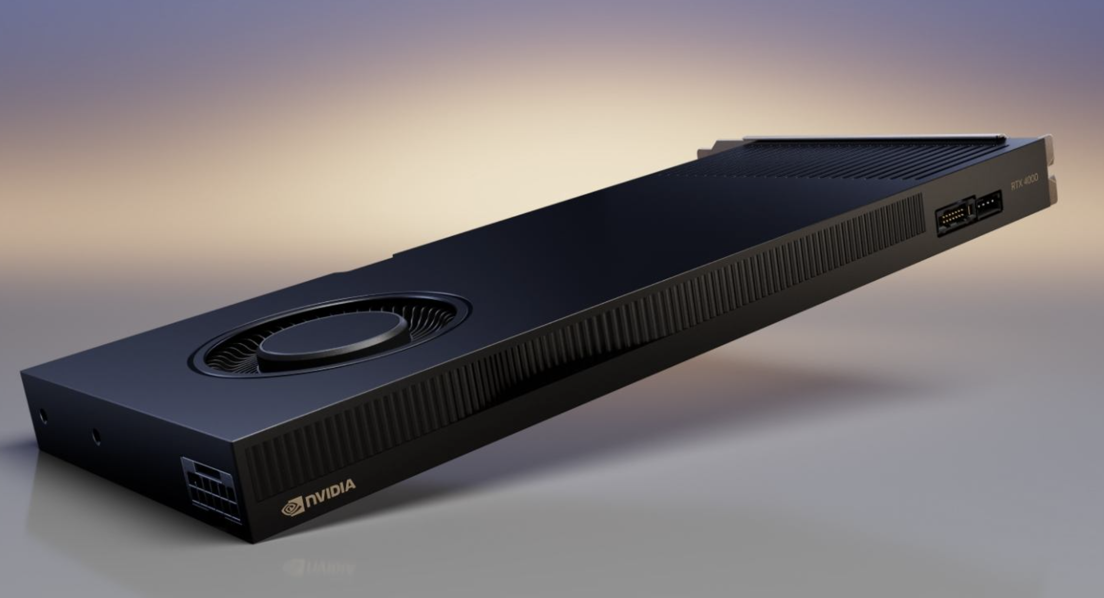
The workstation under my desk is a dual-socket Lenovo with four PCIe-attached RTX A4000 cards. Sixteen gigabytes of VRAM each, 62.40 GiB in aggregate, Ampere, no native FP4 tensor cores. The DeepSeek-V4-Flash-0731 checkpoint on its local disk is 156 GiB. The official model card demonstrates DSpark decoding for this model on a four-GPU GB300 node and recommends specialized MXFP4 backends. I have neither.
The first launch failed before CUDA graph capture. A single-rank FreeToken process asked for a minimum cache plan of 9.14 GB from a remaining device budget of 4.09 GB, and stopped. No launch flag fixes that, so feasibility was a systems problem from the start.
Six weeks later the same machine serves the unmodified checkpoint at roughly 28–30 tok/s on structured code generation, against an approximately 18 tok/s target-only baseline. The work went upstream as three stacked pull requests. The full manuscript, with every measurement, threat to validity, and artifact hash, is available as a PDF. This post is the shorter version, built around the paper’s main architecture figure.
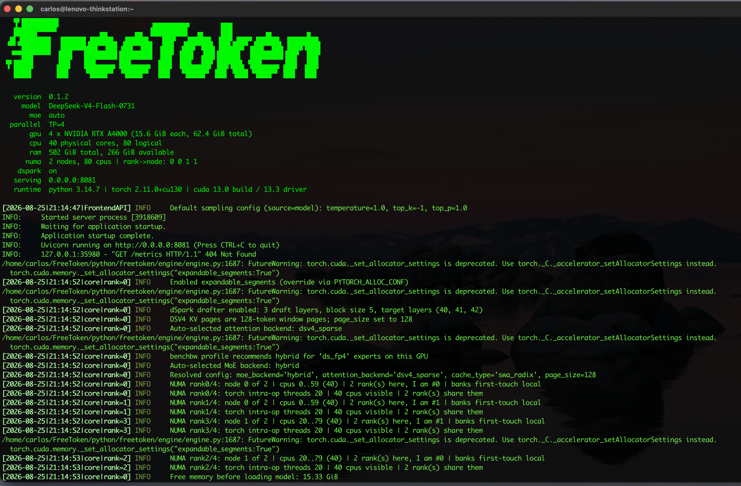
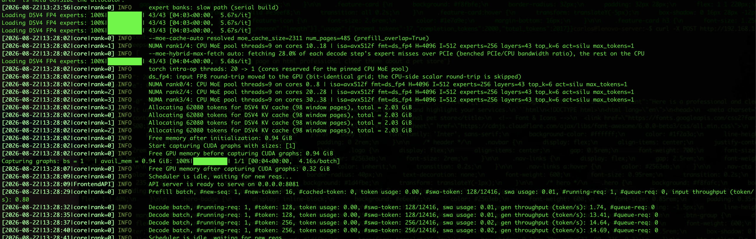
0 0 1 1 that Figure 1 draws. Below it the engine selects its own backends: benchbw profile recommends hybrid for 'ds_fp4' experts on this GPU, then Auto-selected MoE backend: hybrid and the sparse DSV4 attention path. The four NUMA rankN/4 lines report the result of the binding order. Each rank names its node, its 20-core CPU range, and banks first-touch local, meaning its expert pages were written for the first time by a thread that was already pinned to the right socket. Click any log screenshot in this post to read it full size.What FreeToken already does
None of this starts from zero. FreeToken is an edge-native MoE serving system from Yang, Fan, Pan and colleagues at Berkeley and UT Austin, published as arXiv:2608.16157, and its central idea is that a personal machine should be treated as a unified elastic platform rather than as a small GPU. Their overview figure is the design my work sits on top of:
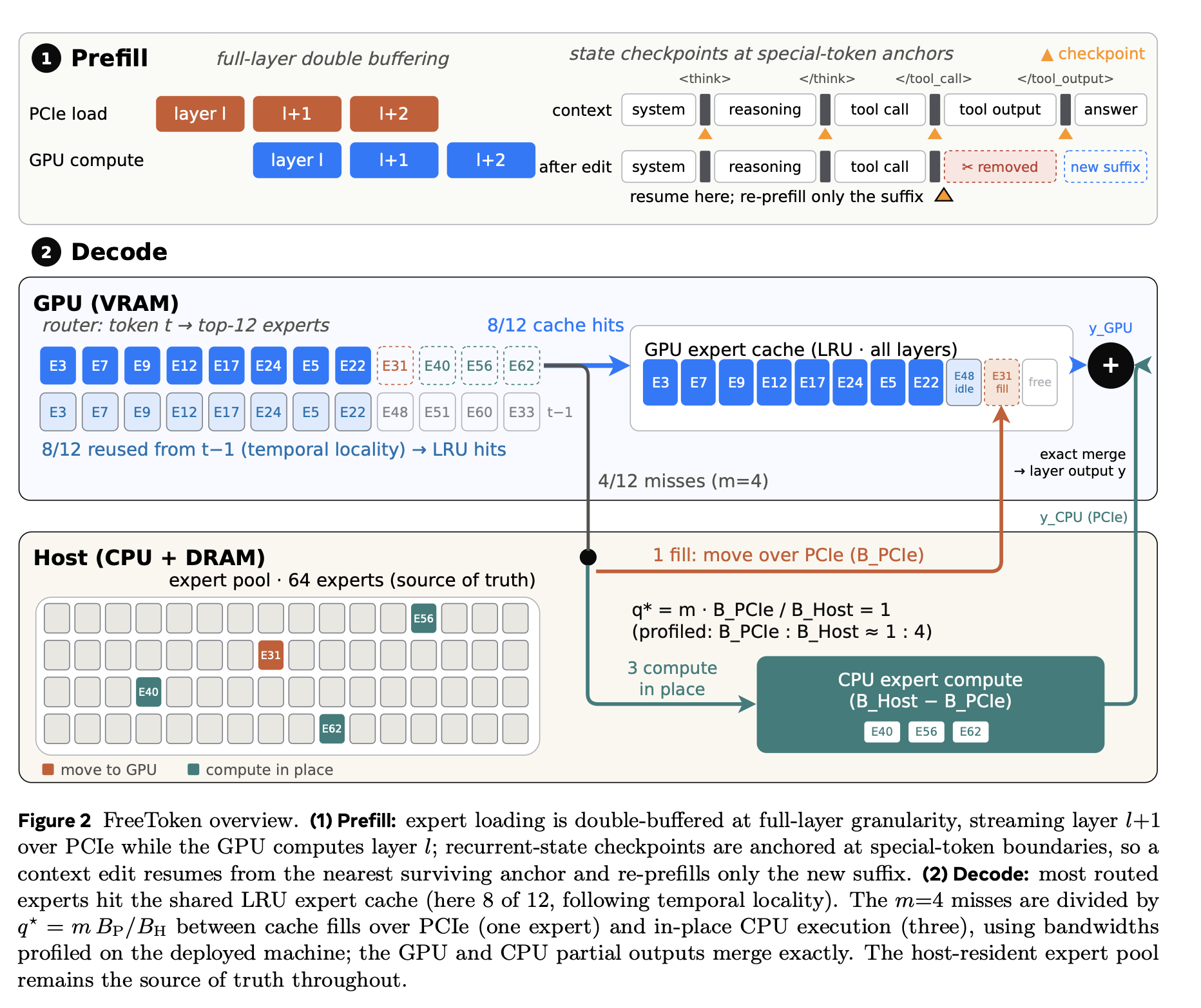
q* = m * B_PCIe / B_Host between one cache fill over PCIe and three experts executed in place on the CPU, using bandwidths profiled on the deployed machine, and the two partial outputs merge exactly. That is the same split rule that lands at 28% on my workstation.Figure and caption reproduced from: S. Yang, X. Fan, M. Pan, H. Xi, Z. Wang, S. Sun, K. Keutzer, S. Han, M. Zaharia, C. Xu, and I. Stoica, “FreeToken: Efficient edge-native MoE serving with bandwidth-adaptive execution,” arXiv preprint arXiv:2608.16157, 2026. [Online]. Available: https://arxiv.org/abs/2608.16157
What that upstream design did not have was a DeepSeek-V4-Flash path that works across four Ampere GPUs with exact DSpark decoding. That is what the three pull requests add, and the rest of this post is the shape of that work.
The architecture, in one diagram
Everything below follows from this figure. It is Figure 1 of my paper, and it shows where each token’s work physically happens on this machine.
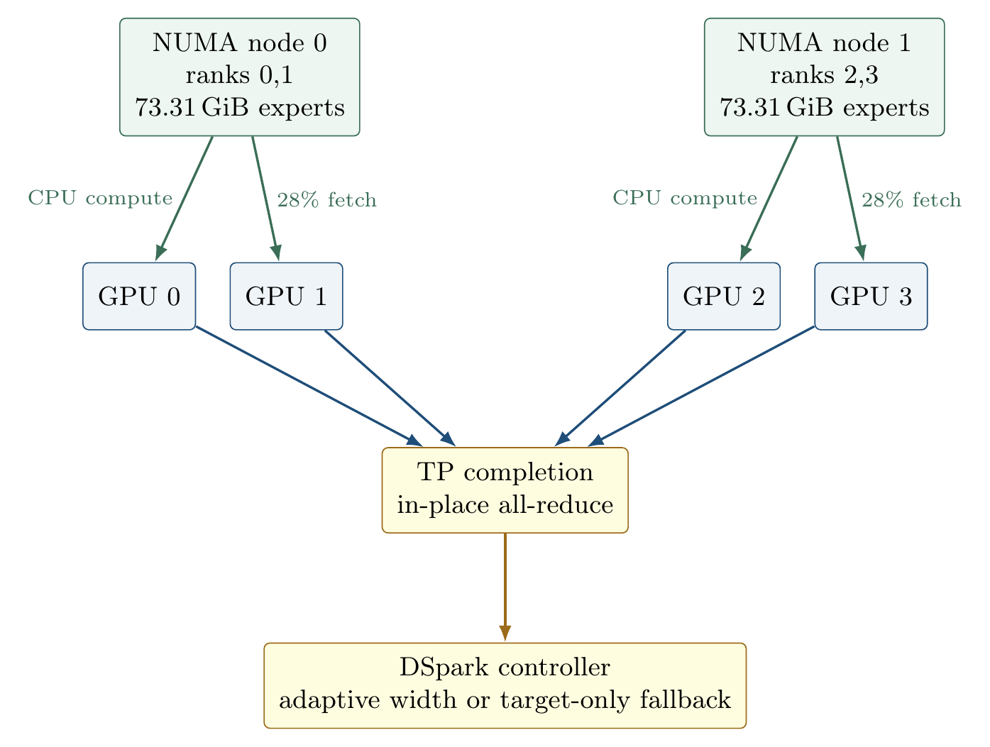
The path runs from top to bottom. Each NUMA node owns 73.31 GiB of routed-expert weights in host memory, first-touched after its ranks are bound to that socket. Ranks 0 and 1 live on node 0 with GPUs 0 and 1; ranks 2 and 3 live on node 1 with GPUs 2 and 3. When a token routes to an expert that is not resident in GPU cache, that miss is split: about 28% of the missing bytes are fetched over PCIe and executed on the GPU, and the rest are executed in place on the CPU by AVX-512 workers reading the packed MXFP4 banks directly. Both paths launch concurrently. The four rank-local partial results are completed by one in-place all-reduce, and the DSpark controller sits on top deciding, per step, how many speculative proposals are worth verifying.
The rest of this post covers why each of those six mechanisms is present.
Why it would not run
The capacity inequality settles the question on its own:
M_{\text{checkpoint}} = 156\ \text{GiB} \;\gt\; M_{\text{VRAM,total}} = 62.40\ \text{GiB}, \qquad \text{ratio} = 2.5
Aggregate VRAM is only useful once a runtime assigns disjoint ownership to the four devices. A single-rank process sees one 16 GiB card, not 62.40 GiB of pooled memory, and setting a tensor-parallel size was not enough by itself, because the then-current DeepSeek-V4 model shapes and loading path assumed one rank and could replicate or retain the largest tensors.
One detail is invisible until you measure it. Slicing a quantized weight with a contiguous narrow() can still return a view, and holding the view holds the entire parent allocation alive. Keeping views instead of cloning into independent storage cost 5.1 GiB per GPU at TP=4. On a 16 GiB device that single line is a third of the budget.
The other rule the loader enforces is that quantized partitioning must preserve blocks. A requested local dimension that cuts an FP4 32-value block, or an FP8 128-value scale grid, is rejected before the model is constructed rather than silently producing garbage. Weights and their scale grids are sliced on the same axis.
MXFP4 is not NVFP4, and the difference matters on Ampere
The routed experts in this checkpoint are packed E2M1 values with one E8M0 scale shared by every block of 32 values. Let c_{b,i} be the four-bit code at position i of block b, let e_b be the unsigned E8M0 exponent code, and let v(c) be the E2M1 lookup value. The decoded weight is
\widehat{w}_{b,i} \;=\; v(c_{b,i})\,2^{e_b-127}, \qquad i = 0,\dots,31
with the E2M1 magnitude set \{0, 0.5, 1, 1.5, 2, 3, 4, 6\} plus one sign bit. Ignoring tensor alignment, a block costs
4 + \frac{8}{32} = 4.25 \ \text{bits per weight}
That is the defining geometry of OCP MXFP4. NVIDIA’s NVFP4 also uses E2M1 values, but with an E4M3 scale per 16 values plus a second-level tensor scale, nominally 4.5 bits per weight before that tensor scale. Calling this checkpoint NVFP4 would be wrong, and it would hide the reason a Blackwell-specific kernel cannot simply be selected on an Ampere card. FreeToken names this expert layout ds_fp4; I call it MXFP4 when I mean the numeric format.
Since the A4000 has no FP4 matrix instructions, the portable GPU kernels read packed nibbles and E8M0 scales directly, decode inside the reduction, and accumulate in FP32:
z_n = \sum_k a_k\, v(c_{n,k})\, 2^{e_{n,\lfloor k/32 \rfloor}-127}
Scales load once per 32-weight block and broadcast. A full BF16 copy of an expert is never materialized, which matters more than the arithmetic rate when the budget is this tight. The CPU path reads the same packed row-major banks with no repack. This is a software execution path for an MXFP4 checkpoint rather than native FP4 arithmetic, and the distinction matters for anyone reading the throughput numbers below.
Where the 28% split comes from
The hybrid fetch fraction in Figure 1 was not chosen by hand. It is the FreeToken rule, instantiated with bandwidths measured on this box. Let B be the bytes associated with expert misses in one step, let q be the fraction fetched over PCIe, and let \beta_g and \beta_c be the achieved PCIe gather and CPU expert-compute bandwidths while both paths run concurrently. The two service times are
T_g(q) = \frac{qB}{\beta_g}, \qquad T_c(q) = \frac{(1-q)B}{\beta_c}, \qquad T_{\text{hybrid}}(q) = \max\{T_g(q),\,T_c(q)\}
With ideal overlap the two paths balance at
q^{*} = \frac{\beta_g}{\beta_g + \beta_c} = \frac{9.85}{9.85 + 25.37} = 0.2797
which is the deployed 28%. The measured inputs matter as much as the formula. Both \beta_c = 25.37 GB/s and \beta_g = 9.85 GB/s were measured under contention. Standalone host-to-device bandwidth on this box is 12.3 GB/s, and using that isolated figure would describe a regime hybrid execution never operates in. The formula is portable; these numbers are not. The 28% is also a machine-calibrated starting point derived from a single-rank profile, while serving runs four ranks with two per socket. Sweeping nearby fractions under the real TP=4 workload is the first item on my list.
First touch, or the banks scatter
Linux places an anonymous page on the node of the thread that first writes it. Load a 36.66 GiB rank-local expert bank before binding the rank, and its pages scatter across both sockets; the CPU expert workers then read remote memory, and PCIe DMA may cross the socket interconnect on the way to that rank’s GPU. The Linux distances here are 10 local and 21 remote, so this is not a rounding error.
The runtime now does this, in order, before any large allocation: read the allowed CPU mask and NUMA CPU lists from sysfs; resolve each CUDA device’s PCI bus ID and its local NUMA node; map ranks to their GPU-local nodes; bind rank CPU affinity and record the placement before affinity hides the original topology; allocate and first-touch the banks under that binding; then split the node’s physical cores among ranks with one coordinator reserved per rank. Each rank ended up with nine AVX-512 expert workers and one coordinator.
The placement reporter runs after CUDA graph capture, not before, so what it prints is the serving state rather than an intermediate loader state:
| Location | Ranks | Expert banks | GPU allocation | CPU |
|---|---|---|---|---|
| NUMA node 0 | 0, 1 | 73.31 GiB | 27.97 GiB | 20 cores |
| NUMA node 1 | 2, 3 | 73.31 GiB | 27.26 GiB | 20 cores |
| Total | 0–3 | 146.62 GiB | 55.24 GiB | 40 cores |
| Share of counted placement | 72.6% | 27.4% |
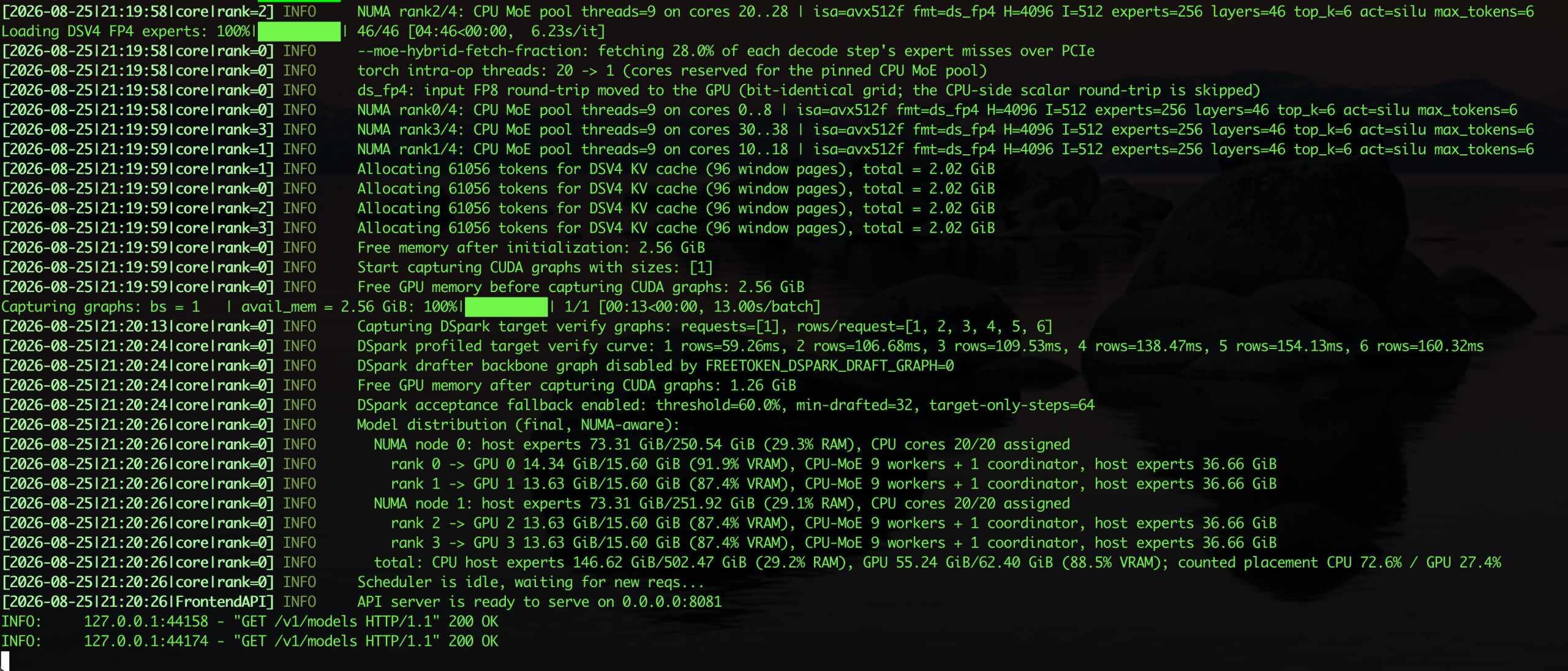
1 rows=59.26ms through 6 rows=160.32ms, where “rows” is the anchor plus k proposals, so one row is width zero. It also prints the fallback thresholds, threshold=60.0%, min-drafted=32, target-only-steps=64, which are the values used in the controller below. The Model distribution (final, NUMA-aware) block is the placement table: 73.31 GiB of host experts on each node, rank 0 at 14.34 GiB of VRAM and ranks 1–3 at 13.63 GiB, nine CPU-MoE workers plus one coordinator each, and a last line summing to CPU 72.6% / GPU 27.4%. This is a 25 August run, so its verify curve sits a couple of milliseconds away from the recorded final configuration charted further down. The shape is the same.Rank 0 used 14.34 GiB and ranks 1–3 used 13.63 GiB each, so the four cards hold 88.5% of their usable VRAM. The host banks take 29.2% of system RAM. Roughly three quarters of this model lives on the CPU side while it is being served.
Speculative decoding that stays exact
DSpark proposes \gamma = 5 tokens per pass with a drafter that ships inside the checkpoint: three MoE draft blocks, a 128-token sliding window, a low-rank Markov head, and a confidence head. Speculative decoding is worth doing because it is exact. The accepted output has the same distribution as target-only sampling. For a proposal x_i,
a_i = \min\left(1, \frac{p_i(x_i)}{q_i(x_i)}\right), \qquad r_i(x) = \frac{\max\{p_i(x) - q_i(x),\, 0\}}{\sum_z \max\{p_i(z) - q_i(z),\, 0\}}
where r_i is the residual distribution the replacement token is drawn from at the first rejection. Both p and q are formed after the request’s temperature, top-p, and top-k policy is applied. Comparing proposals against target argmax would be faster and would bias a temperature-1.0 request toward the mode, so the implementation does not do that. Proposal probabilities, uniforms, first rejection, residual construction, and bonus sampling all stay on the GPU. Exactly two integers cross to the host per step: the accepted length and the emitted target token.
The acceptance rule was not the hard part. The difficulty is that the target verifies anchor plus proposals before it knows the accepted prefix, so a rejection cannot be implemented as a token-buffer truncate. Every piece of state has an owner and needs an explicit rule:
| State owner | Commit | Rejection or unused suffix |
|---|---|---|
| Request token buffer | Accepted proposals plus one target token | Truncate to accepted frontier |
| Target paged KV | Keep accepted rows | Return unused tail pages immediately |
| Draft sliding-window KV | Catch up from committed target rows | Do not advance from abandoned rows |
| SWA slots | Keep accepted positions | Release tail slots immediately |
| Target auxiliary features | Select the accepted physical row | Never commit a rejected feature row |
| Compressor and indexer carry | Commit journal row at accepted frontier | Restore the selected row when later speculative rows overwrote the same ring page |
| Detokenizer | Emit each accepted token exactly once | Stop at EOS or a stop token inside the block |
| Client lifecycle | Preserve owned committed state | Release speculative allocations on disconnect or abort |
The carry journal is the subtle row. Several positions share one 128-token ring page, so releasing whole pages cannot restore an earlier recurrent value inside a page that is still live. The detokenizer row came from a real bug: writing a multi-token block through a single-token path duplicated visible tokens until the contract was fixed to advance engine and tokenizer through the accepted list exactly once.
One more constraint exists only because of tensor parallelism. Every rank must use the same sampling stream and select the same physical graph span. A rank disagreement changes collective ordering and can deadlock the process group, even when each rank’s local token choice looks reasonable on its own.
How many proposals are worth verifying
Let c_i be the confidence, between 0 and 1, that proposal i survives given the previous prefix. Survival through position k and the expected token yield of a width-k verification are
S_k = \prod_{i=1}^{k} c_i, \qquad E(k) = 1 + \sum_{i=1}^{k} S_i
With D the measured draft time and V(k) the median replay time of the target graph for anchor plus k proposals, the one-request scheduler picks
k^{*} = \mathop{\mathrm{argmax}}\limits_{0 \le k \le \gamma} \frac{E(k)}{D + V(k)}
Width zero is legal and still emits one target token; ties keep the smaller width. Measured graph costs are forced monotonic before they enter the selector, so profiling noise cannot make a larger physical graph look cheaper than a smaller one. The measured values:
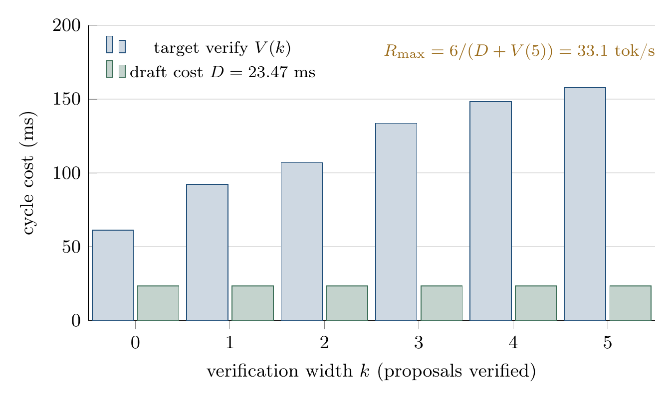
The curve also sets the throughput ceiling. With full five-proposal acceptance a cycle emits six tokens:
R_{\max} = \frac{6}{(23.47 + 157.79)\times 10^{-3}} = 33.1\ \text{tok/s}
and at the 84% acceptance I see on code, a cycle emits 1 + 5(0.84) = 5.2 tokens:
R_{0.84} \approx \frac{5.2}{0.18126} = 28.7\ \text{tok/s}
which matches the 28–30 tok/s region I measure. No amount of confidence-threshold tuning gets this machine to 60 tok/s. Only a substantial cut in draft cost or target verify cost does.
When the drafter stops paying for itself
The width selector runs after the drafter has already executed, so it cannot recover the 23.47 ms of draft cost on a request that keeps rejecting proposals. Structured code is locally predictable and accepts well. Open-ended prose and hard reasoning often do not. A workstation serving one user should not keep paying the draft cost just because the prompt was initially eligible.
The controller watches acceptance instead of guessing from the prompt text. Over a request-local window, with A accepted draft tokens out of G verified proposals, measured acceptance is
\widehat{\alpha} = \frac{A}{G}
Once the window holds at least m verified proposals, the controller sends the request to target-only for C steps when \widehat{\alpha} \lt \tau, and leaves it on DSpark when \widehat{\alpha} \ge \tau. The evaluated settings are \tau = 0.60, m = 32 and C = 64.
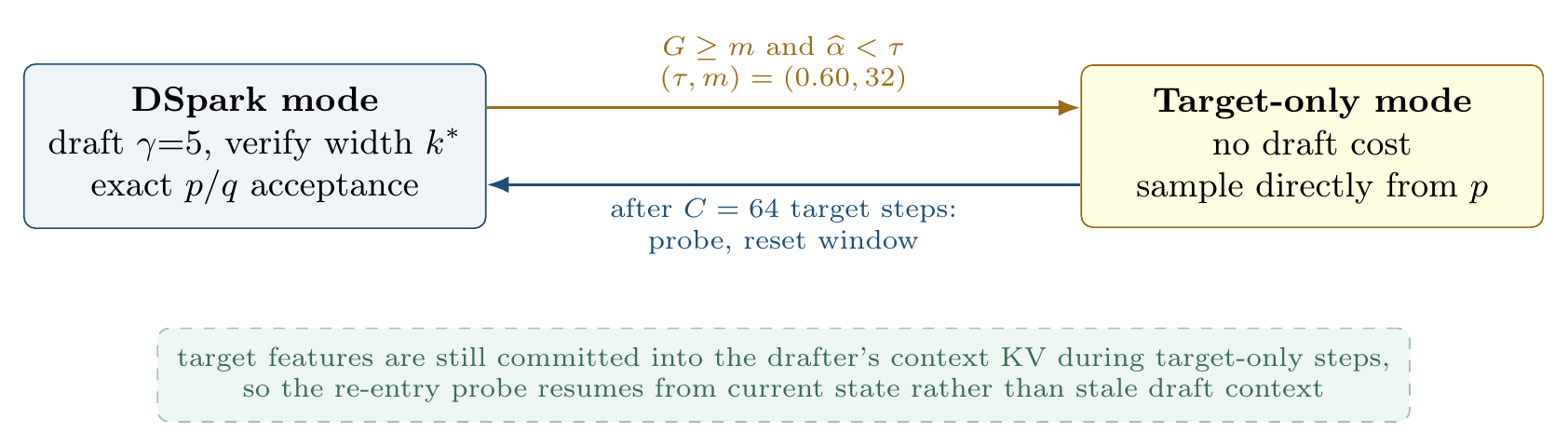
Both modes are target-correct, so switching between them preserves the requested sampling distribution. When DSpark runs, the acceptance and residual rules above are untouched; when target-only runs, tokens are drawn straight from the target distribution. New request IDs reset every counter, so one request can never inherit another’s decision.
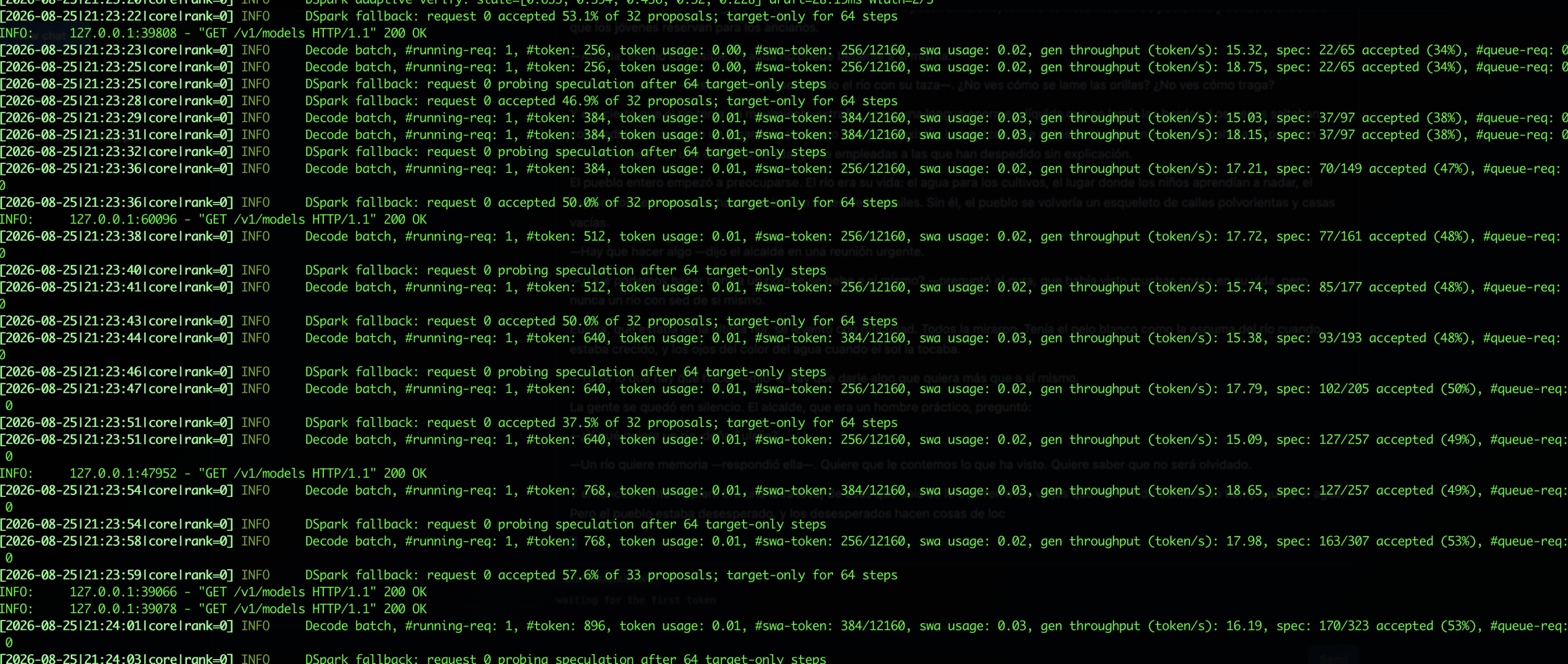
request 0 accepted 53.1% of 32 proposals; target-only for 64 steps is the trip, a full window measured under the 60% threshold, so drafting stops. request 0 probing speculation after 64 target-only steps is the re-entry probe. It trips again at 46.9%, 50.0%, 37.5%, then 57.6%, which is what an unpredictable request looks like: the drafter never becomes profitable, and the controller keeps declining to pay for it. Cumulative acceptance on the right climbs from 34% to 53% as target-only steps dilute the counter, and generation throughput oscillates between roughly 15 and 18.75 tok/s, the mixed and target-only windows from the results table.The composition has four properties: request-local measured acceptance, a bounded target-only interval, drafter-state maintenance during that interval, and re-entry probes. I make no priority claim over other speculative decoders. The checkable claim is that this controller was added to FreeToken’s DeepSeek-V4 DSpark path, tested against its hybrid state machinery, and measured on a workload where the drafter was persistently unprofitable.
Results
Three reporting rules apply to these numbers. Prefill and decode throughput are reported separately, since a short prompt cannot exercise the 2,048-token prefill path. The first status interval after idle time is excluded from steady-state decode, because it contains idle and calibration time. Speculative counters are cumulative since server start, so per-request acceptance is the difference of the counters immediately before and after the request.
| Configuration | Workload | Acceptance | Throughput |
|---|---|---|---|
| Target-only baseline | Reference decode | n/a | about 18 tok/s |
| DSpark PR stack | Structured code | 65–70% | 27.7–29.7 tok/s (1.54–1.65×) |
| Enhanced-v2 + 2048 | Structured code control | 81.6% | 29.29, 30.08 tok/s |
| Enhanced-v2 + 2048 | 25-horses reasoning | 61.0% | 18.37 tok/s mean |
| Fallback enabled | Structured code control | high; no useful trip | 30.55, 27.33 tok/s |
| Fallback disabled | Creative prose | low | about 15.7 tok/s end-to-end |
| Fallback enabled | Same creative prompt | 30.3–59.4% windows | 17.18 tok/s end-to-end |
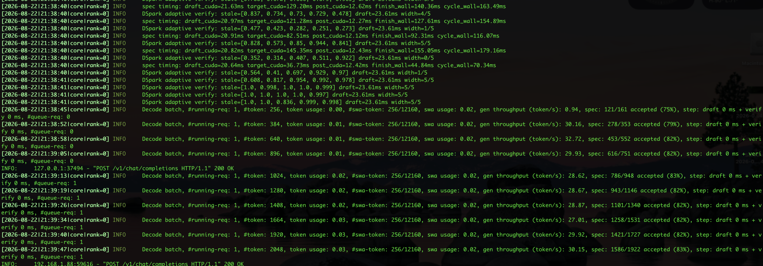
The structured-code improvement is the primary gain: 27.7–29.7 tok/s against an approximately 18 tok/s target-only baseline, with later controls reaching about 30 tok/s at higher acceptance. The fallback result is narrower. One matched creative request improved from about 15.7 to 17.18 tok/s, a 9.4% rate increase, with wall time falling from about 98 s to 88.07 s for 1,513 tokens. During fallback the target-only windows reached 17.86–19.59 tok/s. That is one matched run, with the baseline wall time inferred from server timestamps and slightly different natural completion lengths. It is evidence for the controller, not a workload-wide average.
The largest confirmed wall-time improvement came from doubling the default prefill chunk.
| Chunk size | Full-chunk throughput | Total prefill wall time |
|---|---|---|
| 1,024 tokens | 321.8–323.2 tok/s | 25.79 s |
| 2,048 tokens | 625.4–627.3 tok/s | 15.31 s |
| Change | about 1.94× | 40.6% lower |
That gain comes from denser prefill work and better amortization, not from the fallback. A separate 9,139-token prompt with a 200-token response completed coherently without OOM. A faster chunk is worthless if it crosses the workstation’s graph or activation budget.
The results that did not work
Graphing the drafter did essentially nothing. A matched A/B on the same commit put the captured drafter backbone at 25.03 tok/s end-to-end against 24.78 eager, and the steady mean favored eager, 24.23 against 23.97. Capture reduced the drafter substage from about 21.71 to 18.43 ms, but jitter rose from 3.72 to 4.84 tok/s standard deviation, and fallback entries rose from 7 to 12. Both outputs were coherent. The deployed service keeps the eager drafter, with graph replay behind an opt-out switch until repeated tests explain the variance.
More cache is not monotonically better. A 0.90 memory ratio auto-sized 2,509 MoE cache slots and left 1.02 GiB before graph capture, at which point DSpark verification capture failed with OOM. A 0.80 ratio selected 2,016 slots, left 2.56 GiB before capture and 1.26 GiB after, and started. Residency competes directly with the reserve that graph capture needs.
Reasoning termination is still a real failure. Bounded bridge-and-torch prompts found the correct strategy without repetition, then consumed a 1,200-token budget formalizing the proof and never entered the final answer channel. A 25-horses run found the correct seven-race strategy and was cut during its lower bound. Correct intermediate reasoning that never reaches an answer is a serving-quality bug, and output budgets and termination behavior need their own fix.
Concurrency is not claimed at all. Adaptive width selection here is specialized to one active request. Padding every request to a single maximum width is not equivalent to a global capacity decision across flattened variable-length requests, so there is no multi-request throughput number in this work.
Making it a service
The model did not become a service when the first correct token appeared. Some of what stood between those two states:
- Compiler. The workstation’s default GCC 16 was newer than the CUDA JIT would accept, so the service pins NVCC and host C++ to GCC/G++ 15.
- KV capacity. The validated deployment allocates 477 full-KV pages, or 61,056 tokens of prompt plus output. The architecture supports far more context than that. An architecture limit and an allocated workstation capacity are different quantities and should not be quoted interchangeably.
- Loading and rendezvous. Expert loading is serial under the proven profile, and the distributed startup timeout is 1,800 s to tolerate legitimately skewed rank-local bank loading.
- Readiness. The HTTP frontend binds before the expert banks finish loading, so the manager waits for the engine’s
ready to serverecord instead of treating an HTTP response as model readiness. - Teardown. TP workers are detached multiprocessing children and can retain the rendezvous port after the frontend stops. The management script resolves only service-specific ranks and shared-memory objects, and never terminates by broad process-name match.
- Provenance. Source changes reach the Lenovo checkout only through a named branch pushed to the fork, then fetch, switch or fast-forward, then server-side tests at that exact commit. Copying source files directly into the server is outside the validated procedure.
These items are part of the feasibility result. A model that starts only after manual process cleanup, or that OOMs on a long prompt right after a clean benchmark, is not a reproducible deployment.
The upstream stack
Three stacked PRs against FlashML-org/FreeToken, reviewed in the order 1/3, 2/3, 3/3 even though GitHub numbered the second layer #69 and the foundation #70. These are cumulative diffs, so a stacked PR includes its prerequisites and the rows must not be summed:
| Order | Pull request | Head | Commits | Files | Added / removed |
|---|---|---|---|---|---|
| 1/3 | #70, TP runtime | c066b38 | 6 | 18 | 903 / 121 |
| 2/3 | #69, exact DSpark | 2cf938b | 8 | 53 | 5,360 / 193 |
| 3/3 | #71, adaptive verification | 4800af0 | 18 | 73 | 7,465 / 335 |
PR 1 is deliberately independent of DSpark. Its only job is to make one target-model forward mathematically complete and memory-feasible across four ranks. PR 2 loads the checkpoint drafter, builds draft context KV, verifies a block, and implements exact greedy and probabilistic acceptance, then fixes what only appears under full hybrid serving. PR 3 is where the correct implementation becomes a measured runtime: adaptive TP verification, GPU-resident probabilistic sampling, exact multi-token detokenization, fused hyper-connection normalization, long-prefill bounds, in-place NCCL, placement reporting, route-aware expert fetch, and the fallback.
Two GPU-side changes in PR 3 need credit and caveats. The fused hyper-connection pre-normalization reads the BF16 source once and accumulates squares in FP32, instead of materializing a full FP32 copy plus a second FP32 square tensor. On an RTX 6000 Ada microbenchmark at the DSV4 hidden geometry, the T = 8192 operation fell from 1.944 to 0.304 ms, a 6.4× kernel speedup. That optimization originated with Gabriel Devenyi’s FreeToken PR #101; my change extends it to the DSpark drafter and adds long-prefill bounds. The Ada microbenchmark is not an A4000 end-to-end result. Separately, TP all-reduce now operates in place on its contiguous input, removing the two device copies the older symmetric-staging path performed around every reduction. That path had dominated an earlier TP=4 verification trace on this PCIe configuration.
At submission the complete three-PR stack passed 192 focused DSV4 tests on the TP=4 server, and the fallback lineage passed 202 DSpark and hybrid-fetch tests at its exact pushed commit. Coverage runs from TP=1/2/4 shape ownership and quantization alignment, through greedy and sampled acceptance including residual recovery and width zero, to paged KV, SWA, recurrent carry, and client-disconnect cleanup.
What made it feasible
No single optimization explains this. MXFP4 shrinks expert storage, and the checkpoint still exceeds aggregate VRAM. CPU offload adds capacity, and a single PCIe expert miss can dominate a short decode step. Tensor parallelism adds VRAM, and it also adds collectives and creates four host-memory consumers. DSpark amortizes target work, and low acceptance can make its draft cost counterproductive. NUMA binding improves locality, but only if it happens before first touch. CUDA graphs cut launch overhead, but only if fixed buffers and state ownership survive replay.
The feasibility chain is conjunctive:
\begin{aligned}\mathcal{F} = \ &\text{rank-local storage} + \text{MXFP4 execution} + \text{NUMA-local banks} \\ &+\ \text{hybrid miss service} + \text{exact speculative state} + \text{bounded graph memory}\end{aligned}
Remove any one term and you either break correctness, exceed memory, or leave a large avoidable latency on the table. Each of those ideas has prior work behind it: tensor parallelism, speculative sampling, paged state, microscaling formats, offload, CUDA graphs, NUMA placement, and the bandwidth-adaptive MoE execution that FreeToken contributes. DSpark supplies the trained drafter and the confidence-scheduled verification. The contribution is at the integration boundary, where these mechanisms have to agree about tensor ownership, quantization metadata, speculative state, rank-local memory, PCIe service, graph replay, and request lifecycle.
The scope is one machine, one active request, limited repetitions, and qualitative output checks rather than benchmark accuracy or human preference studies. The bandwidth split formula is portable; its measured inputs are not. The case study shows something narrower than a speed number: a 156 GiB MXFP4 checkpoint becomes practical on 62.40 GiB of Ampere VRAM when memory ownership, numeric format, speculative correctness, PCIe service, and NUMA locality are designed together rather than separately.
The full manuscript, with the complete ownership table, the threats to validity, and the reproduction checklist, is here as a PDF.
References
S. Yang, X. Fan, M. Pan, H. Xi, Z. Wang, S. Sun, K. Keutzer, S. Han, M. Zaharia, C. Xu, and I. Stoica, “FreeToken: Efficient edge-native MoE serving with bandwidth-adaptive execution,” arXiv preprint arXiv:2608.16157, 2026. [Online]. Available: https://arxiv.org/abs/2608.16157